How Quantexa's Entity Quality Overlinking (EQO) Model Quantifies Entity Resolution Accuracy
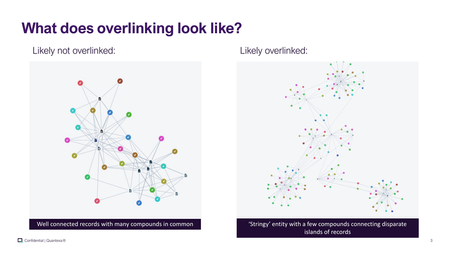
Why entity quality is a problem worth modelling Entity resolution (ER) is the backbone of Quantexa's platform: it takes millions of raw records from different source systems and links the ones that refer to the same real‑world entity (a person, a business, etc.) into a single resolved entity. Records are linked when they share compounds — normalised keys built from attributes such as name + address, name + phone, or name + date of birth. Any linkage system must navigate the following two failure modes: Overlinking — a compound key pulls together records that actually describe different real‑world entities, producing a false positive merge. Per the Quantexa glossary, overlinking "occurs when a Compound Key brings together separate Records that describe different Entities … typically caused by similarities between the Records of different Entities." Underlinking — the opposite failure: keys are so strict that records belonging to the same entity never get joined (a false negative), usually because of missing or mistyped data. Note that an entity can be simultaneously over and underlinked at the same time. This post is about the first of these. Overlinking is insidious because a single over‑merged entity can quietly corrupt everything built on top of it: network graphs, risk scores, alerting, and — in a financial‑crime context — the picture an investigator forms of who is connected to whom. If two unrelated businesses are fused into one entity, every downstream analytic inherits that mistake. The challenge is that ER runs at enormous scale. You cannot manually inspect hundreds of millions of entities to find the bad merges. Entity Quality Overlinking (EQO) is Quantexa's answer: a machine‑learning model that assigns every resolved entity an Entity Quality Overlinking Score (EQOS) between 0 and 100, where 0 means bad quality (overlinked) and 100 means good quality (not overlinked). It lets you sort a whole population by quality and attack the worst offenders first. What overlinking actually looks like Before modelling anything, it helps to build visual intuition for the signal. Two entities are depicted below in terms of their records and compounds: Two archetypes emerge: Likely not overlinked (left): a dense, well‑connected entity. Most records share compounds with most other records. The entity is internally consistent — it looks like many observations of one thing. Likely overlinked (right): a "stringy" structure — several dense clusters (each a genuine sub‑entity) joined by a few thin bridges. Those bridges are the tell‑tale sign that one or two coincidental compounds (a shared address, a recycled phone number) have welded distinct real‑world entities together. What does EQO do? EQO generates a prediction for each entity for how overlinked it is. It has primarily been tested on Businesses and Individuals, but it can be run on other entity types too. How well does it work? On held‑out UK data the following accuracy is achieved: Entity type Accuracy (UK) Business ~80% Individual ~90% In conclusion, EQO can accurately predict whether a given entity that has been formed through Quantexa's entity resolution is overlinked or not.37Views0likes0CommentsIntroducing Network Features Can Help Your Organization Detect Risks at Speed
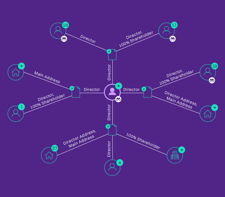
The importance of context In the world of risk modelling, the input data points (or features) are particularly important – usually even more important than the choice of model or algorithm. In an industry with significant regulatory pressure for transparency and explainability in modelling, model choice is often restricted meaning the choice of input features can be the core reason for success (or failure) of the model. So, the key question is – how can we bring as much context into our features as possible? Network-based features provide an excellent way to inject a huge amount of information into your model, whilst keeping the required transparency and explainability. One way of achieving this is by using bespoke document-entity networks to generate features describing how businesses and individuals are related to each other. At Quantexa, we’ve used network features describing relationships between companies and their directors as key inputs into our Shell Company detection model, which has resulted in a 20% uplift in performance compared to using just record-level features. The model output – predicted shell companies and the incorporating agents creating them – has a range of applications for enhanced risk detection across AML (Anti-Money-Laundering), KYC (Know-Your-Customer), Risk and Fraud. Introducing network features Networks can be used to model relationships between entities in many different circumstances. For example, networks of payments between parties can be used to find signs of financial crime. Searching for certain shapes in the network (e.g. cycles of similar sized payments) can lead to the detection of risks that would not have been identifiable by looking at transactions in isolation. Simple characteristics such as the size of a network, the number (or density) of connections, and the number of layers can all be useful dimensions for segmentation or feature generation. The power of networks in machine learning In the Quantexa Shell Company detection model, we have used a combination of features derived from organizations’ wider networks (including their legal hierarchies and director networks) and from company registry records. These network features include the identification of network shapes and patterns, as well as using techniques from graph analytics (including centrality analysis) to create new information about the entities in the network, like finding directors with high importance in the network. The director in the network has control of four organizations, all with single shareholders and based in profligate (or highly connected) addresses. Creating features such as ‘director’s company is based at a profligate address’ and ‘director shares directorship with a 100% shareholder’ can be very informative in finding shell companies. In addition, the director above has high ‘page rank’ (centrality) in the wider network. These new network characteristics are used as features within a company-level model. This evaluates if each company is likely to be a shell based not just on its own characteristics (size etc.) but also on this network context. Including network features in the model significantly enhanced its performance and has so far led to the identification of over ten thousand new shell companies not identifiable from record-level models alone. The use of network features to provide context has added significant value in other areas too, including scorecard tuning, and even data quality analysis.27Views0likes0Comments
Getting the Most from Q Knowledge Graph Perspectives
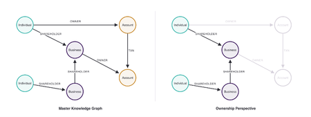
A Knowledge Graph typically contains rich information about multiple domains. This can be extremely valuable for insights, but in practice the size and density of data in knowledge graphs can make analysis difficult. With Quantexa’s Entity Resolution, you can build a network of linked Entities from a wide range of different documents. For example, we could find business, individual and account Entities across internal customer data, corporate registry information and sanctions lists. These Entities will be linked by different relationships, such as shareholdings, ownership and transactions between accounts. This network can act as a single source of truth for your data, though it is likely to be incredibly large, with millions or billions of nodes and edges. For many analytical use cases, creating a Knowledge Graph is a first step in making this data more accessible. A Knowledge Graph can be created from these big networks by treating Entities as nodes, and relationships as edges. Different node and edge types can be used to represent distinct types of Entities and relationships. Because a Knowledge Graph represents a full view of data from Entity Resolution, only some nodes and edges may be relevant to specific analysis. For example, transactions may be irrelevant for analyzing circular ownership of businesses. In a similar fashion, shareholding information may be irrelevant for analyzing certain transaction patterns. Exploring the whole Knowledge Graph for either of these use cases can result in inefficient use of compute resources when querying the Graph, and at worst, can result in subtly incorrect results and conclusions. To resolve this issue, we can use Q Knowledge Graph Perspectives. A Perspective is a derived view of the original Knowledge Graph, defined in such a way to focus on specific, relevant information for an analytical question or use case. Importantly, we can derive as many Perspectives as there are use cases, each representing the original Knowledge Graph in a way that maintains the most relevant nodes and edges. Here we will explore two ways Q Knowledge Graph Perspectives can be used: To filter a Knowledge Graph (keeping only relevant nodes and edges) To augment a Knowledge Graph (deriving implicit edges not originally present) Filtering the Graph Let’s return to an example where we want to perform analysis of company ownership within our Graph. We can use a Perspective to narrow the Graph down to a subset of important node and relationship types. The original Knowledge Graph (left) and an ownership Perspective derived from it (right). Only shareholder edges are kept. Accounts, account ownership, and transactions are dropped, since they are not relevant for this specific analysis. This has implications for efficiency of Graph querying and analysis. Running our ownership-related queries across this Perspective means that the Graph is smaller and cheaper to traverse, particularly if we don’t define extremely specific node and edge types in our queries. In addition, there is no additional storage cost for this new graph, because Q Knowledge Graph Perspectives reference the original knowledge graph data matrices wherever possible, rather than writing new copies. Less obviously, but often more importantly, it stops irrelevant structure influencing your results. Certain Graph algorithms will treat different node and relationship types as equal, which may not be desirable if trying to answer specific questions. While deriving Graph structure through Entity resolution of multiple data sources provides a solid data foundation, the calculation of e.g. PageRank to explore shareholding patterns specifically, would be unduly influenced by the presence of other irrelevant data, e.g. payment flows (Fig. 1). Without filtering the Graph for the relevant nodes and edges, PageRank could output misleading results and be used to draw incorrect conclusions. Here, Perspectives help to narrow the focus of graph analytics, to answer contextual questions about your data. Making implicit relationships explicit While filtering the graph is useful for many analytical use cases, there are some where the actual relationships and patterns we want to explore are not yet present in a knowledge graph. Rather than filter, we might want to alter the schema of a knowledge graph through derived edges, which has separate implications for scalability and analytical inference. A payments Perspective. Wherever an Individual owns an Account that transacts with an Account owned by another Individual, a new ‘payed’ relationship is created between the two Individuals. The Account nodes are no longer required and are dropped. We can use Perspectives to add new edges to a knowledge graph, through augmentation. With augmentation Perspectives, we can specify a schema pattern that we want to replace with another. For example, if we want to explore transactions between Individuals in our knowledge graph, rather than operate on a graph containing account ownership, we can directly augment the graph to create relationships directly between these Individuals, where a payment has occurred (Fig. 2). Q Knowledge Graph achieves these schema alterations through matrix multiplication, making these operations lightning fast when compared to other Graph Database solutions. There are several advantages when using this Perspective for Individual-based payment analytics. The knowledge graph is now effectively ‘compressed’, containing only relevant nodes and edges for this specific use case. Any graph algorithms running over this augmented Perspective now have fewer ‘hops’ to traverse, reducing their run time and computational cost. Similarly to the filtering example, there is also an advantage in terms of graph algorithm result interpretability. When looking at payment chains between individuals, we might care less about e.g. how many Accounts an Individual owns, and more about the flow of funds from one individual to others. The removal of irrelevant Account nodes here will prevent confusing results from graph algorithms like centralities and community detection, that are heavily influenced by the structure of a graph. Building Perspectives: a worked example In the following worked example, we build a knowledge graph and derive two Perspectives from it. Creating a Knowledge Graph Here, our Knowledge Graph has been created through the output of Quantexa’s Batch Resolver entity resolution. It has three Entity types and six relationship types, spanning both ownership and payments. import qknowledgegraph as qkg kg = qkg.KnowledgeGraph.load("kg.kginfo", spark) kg.overview() Figure 3. The metagraph (knowledge graph schema) of our knowledge graph. Perspectives can be defined by working directly with the metagraph. In Q Knowledge Graph you define a Perspective by manipulating the metagraph (Fig. 3). You can define a Perspective, and sketch the modification to the metagraph to validate that you have made the intended changes, before running Perspective generation. Once you’re happy, you can apply the Perspective to the knowledge graph and save it to disk. An ownership Perspective, by filtering ownership_mg = kg.metagraph.select_triplets( "individual-shareholder-business", "business-shareholder-business", ) ownership = kg.save_perspective( ownership_mg, name="ownership", output_root=OUTPUT_ROOT, ) Figure 4. The ownership Perspective metagraph. Faded node and relationship types will be dropped upon running Perspective generation. A payments Perspective, by augmenting Here we declare the path we want to collapse, name the relationship it produces, and then keep only Individuals. from qknowledgegraph.triplet import Triplet ind_owner_acc = Triplet("individual", "owner", "account") acc_txn_acc = Triplet("account", "txn", "account") payments_mg = kg.metagraph.augment( ("pays", [ind_owner_acc, acc_txn_acc, ind_owner_acc.invert()]) ).select_nodes("individual") payments = kg.save_perspective( payments_mg, name="payments", output_root=OUTPUT_ROOT, remove_self_loops=True, ) Note that remove_self_loops=True makes a difference to the Perspective result. Without it, every Individual who moves money between two of their own Accounts will be represented as paying themselves, which may or may not be desirable for different graph algorithms and analysis. Figure 5. The payments Perspective metagraph. The dotted pays edge is derived, and everything it was derived from has been dropped. Perspectives in practice To demonstrate the impact of using Perspectives, we generated a graph using the same schema as in the examples above. The knowledge graph contains one million nodes and 5.4 million edges, made up of 400,000 Individuals, 100,000 Businesses and 500,000 Accounts. We then build both types of Perspectives mentioned above and run the same analysis on each. Nodes Edges Density Mean degree Perspective build time Original Graph 1,000,000 5,449,319 5.45 10.9 - Ownership Perspective 500,000 749,636 3.00 3.0 <0.1s Payments Perspective 400,000 1,961,300 12.26 9.8 0.4 s Both the ownership and payments perspectives have drastically different structural properties (Table 1). As well as being smaller, their density and degree distributions are different to the original knowledge graph. It is important to remember that these structural changes will have strong implications for analytics and graph algorithms. Summary When working with complex graph data, a good pattern is to create one ‘master’ Knowledge Graph, and derive several Perspectives that each suit a particular set of questions and analyses. Perspectives help to focus analytics on nodes, edges and patterns in your graph data that are relevant to specific use cases. Using Perspectives smartly can unlock insights that are difficult to spot in rich, dense graphs.66Views0likes0CommentsCreating and Exploring a Q Knowledge Graph
Organisations today hold more data than ever, but most of the value does not come from the individual records, but in the connections between them. Which individuals sit behind a cluster of businesses, forming shell networks? Which accounts move money between each other to hide a fraud ring? These are network questions, and answering them means treating your resolved data as a graph. Traditional graph databases work well with small graphs, but they tend to struggle once a network grows to hundreds of millions - or billions - of nodes and edges, which is exactly the scale of real data problems organisations try to solve. That's exactly what Q Knowledge Graph (QKG) is for. It’s built to run algorithms and perform analytics efficiently, effectively unlocking graph data science at scale. In this article we'll cover the why, the what, and the how of building your knowledge graph and introduce how to explore it to find insights. Background Quantexa's Entity Resolution turns messy, scattered data into a connected network of entities. You can bring together internal customer records, corporate registry and sanctions lists, and resolve these records into entities - for example business, individual, address, account - linked through the relationships that connect them in the real world: shareholdings, ownership, and transactions between accounts. The result is a single source of truth for your data, which is also enormous - often millions or billions of nodes and edges. That scale is exactly why a Knowledge Graph is usually the next step for many analytical applications. A knowledge graph is a type of graph that shows the relationships between different pieces of data. It represents a network of real world entities and the relationships between them. What is a Q Knowledge Graph? Q Knowledge Graph is our in-house graph processing engine and framework, designed to query and analyse knowledge graphs generated from Quantexa. It offers a network science friendly Python API and native support for Graph Machine Learning, all running very efficiently at scale thanks to a sparse-matrix backend built on distributed linear algebra. A node is typically a resolved Quantexa entity - an individual, a business, an account, a telephone - or a document. Each node type carries its own features (numeric or string attributes). Relationships are typed and directed. Edges are written as head-relationship-tail triplets. individual-owner-account and account-txn-account are two different relationship types, and QKG keeps them distinct. In code, that edge is a first-class object: import qknowledgegraph as qkg qkg.Triplet("individual", "owner", "account") # (head, relationship, tail) qkg.Triplet.from_string("individual-owner-account") # the same, as a string The full set of node types and relationship types represents the graph's schema, which is called the metagraph - more on that when we start exploring. Why use QKG? QKG is built specifically for graph analytics on Quantexa resolved data, at scale, and without leaving the Python ecosystem. A few things it gives you: Network science on Quantexa data, without leaving Python. You can run complex graph operations - such as centrality, ego network expansion, cycle detection and more - directly against your resolved entities. A bridge to graph machine learning. QKG can shape neighborhoods and hand them straight to PyTorch Geometric to train GNN models. Scale. Sparse matrices plus Spark for the heavy joins mean the same code works on a toy graph and on a production-sized one. Pluggable backends. SciPy out of the box, GraphBLAS for acceleration, or NetworkX when you want interoperability - switchable without rewriting your analysis. Getting started The snippets below are written to be run interactively in a Jupyter notebook. Everything assumes a Spark session, which you can start up using the below QPython function: from qpython.qspark.spark import start_spark spark, _, _ = start_spark("qknowledgegraph") import qknowledgegraph as qkg Creating a graph There are several routes into QKG, depending on where your data is stored. The fastest way to get a real graph to play with is a generator. These write a proper graph to disk and hand you back a KnowledgeGraph: kg = qkg.generators.gen_individual_business_txn_graph("./data", director_density=0.1) That's it - you now have individuals, businesses and accounts, and multiple relationships between them. To reopen a saved graph later: kg = qkg.KnowledgeGraph.load("./data/simple-graph.kginfo", spark) You can also feed in the Quantexa Batch Resolver output. You need to point QKG at Batch Resolver outputs and declare which entities, edges and features you want to keep: import qknowledgegraph.ingest.qbatchresolver as qbr from qpython.qbatchresolver.batch_resolver import BatchResolver br = BatchResolver("path/to/batch_resolver/") kg = qbr.KnowledgeGraphCreator( qbr.NodeExtractor("business", F.col("isOnHotlist").cast("float")), # keep a feature qbr.RelationshipExtractor("relationship"), qbr.RelationshipExtractor("role", source="individual", target="telephone"), ).create(br, output_root="./data", graph_name="qbr", parquet_write_mode="overwrite") NodeExtractor and RelationshipExtractor - define which node types to keep, which features to carry over, and which edges to build. Using this information, KnowledgeGraphCreator(...).create(...) runs the ingest. Exploring a graph Let's first take a look at the generated knowledge graph. Running the following code snippet will sketch the graph's schema (every node type and the relationship types connecting them) as a diagram: from qknowledgegraph import viz viz.draw_metagraph_pydot(kg.metagraph) You can then explore the created knowledge graph by running the code below: kg.overview() # node & edge counts list(kg.entities) # node types [t.motif_string for t in kg.triplets] # relationship types This will print the summary of the graph, as you can see in the below image. Reshape it with Perspectives Most of the times, knowledge graphs are heterogeneous - they contain multiple types of nodes and edges. However, often only some nodes and edges may be relevant to your Knowledge Graph. For example, if you're tracing how money moves between people, the transaction edges are what you need and the address links are just noise; on the other hand, transactions may be irrelevant for analysing corporate hierarchies. Using the Quantexa’s patented Perspective technology, you can easily transform the graph via the metagraph, for example by collapsing a multi-hop path into a single derived relationship, then pruning down to just the nodes types you care about: def txn_path(src, dst): return [ qkg.Triplet(src, "owner", "account"), qkg.Triplet("account", "txn", "account"), qkg.Triplet(dst, "owner", "account").invert(), ] end_nodes = ["business", "individual"] transaction_paths = [txn_path(src, dst) for src in end_nodes for dst in end_nodes] mg = kg.metagraph.augment(*[("txn", path) for path in transaction_paths]).select(nodes=["business", "individual"], relationships=["txn"]) Similarly as above, by running the code viz.save_metagraph_pydot(mg, show_change_from=kg.metagraph, path="./mg_diff.png") viz.draw_metagraph_pydot(mg, show_change_from=kg.metagraph) you can visualize the metagraph of your transformed knowledge graph after augmentation and pruning, as shown below. You can finally save the new metagraph by running the below code perspective = kg.save_perspective(mg, name="perspective", output_root="./data") Rank the important nodes With a graph in hand, you can run complex algorithms such as PageRank, which gives you back the most relevant nodes (in this case individuals) in your graph. pagerank = qkg.PageRank(perspective).run() Now we print the top 5 most important individuals found with PageRank. top_individuals = ( pagerank.pandas().get("individual") .sort_values("pagerank", ascending=False) .head(5) .assign(entity_type="individual")[["entity_type", "graph_node_id"]] ) Build ego-networks EgoBuilder grows a neighbourhood outward from seed nodes, following a path query (head-relationship-tail, with * for "any" and | for "or"): ego = qkg.EgoBuilder(perspective).seed(top_individuals).expand("individual-*-business-*-individual") print(ego.explain()) # see the planned expansion before it runs nhds = ego.run("./data/nhds") # nothing runs until .run(); returns a Spark DataFrame The length of the path query controls how many hops the expansion travels from each seed. Each -relationship-node segment you chain on is one more hop outward: individual-*-business-*-individual is a two-hop expansion (individual → business → individual), whereas individual-*-business would stop after one. The more hops, the wider -- and more computationally expensive - the neighbourhood. Seeds can be a node type, a list of types, or a DataFrame - so you can, for example, seed the expansion with your top PageRank nodes. Ask questions in Cypher If you prefer a query language, CypherInterpreter runs OpenCypher-style MATCH ... RETURN queries over neighbourhoods: from qknowledgegraph.cypher import CypherInterpreter seeded = qkg.EgoBuilder(kg).seed("individual") CypherInterpreter(seeded).run( "MATCH (:individual)-[]->(biz:business)-[]->() RETURN biz.x1", neighborhood_transform=inject_business_features ) The neighborhood_transform parameter lets you inject the features (in this case business features), in order to extract the x1 feature. From Ego-networks to Scoring Graphs Ego-networks can be converted to NetworkX graphs for custom graph analysis, or to Quantexa ScoringGraph objects for the Assess scoring pipeline. from qknowledgegraph.neighborhood.scoring import neighborhood_df_to_scoring_graphs scoring_graphs = neighborhood_df_to_scoring_graphs( nhds, output_path="./data/scoring_graphs", mode="overwrite" ) scoring_graphs.scoring_graph.show(5, truncate=True) The ego-networks around our highest PageRank individuals are now Quantexa Scoring Graphs, ready for network scoring rules in an Assess pipeline. Summary This article is a brief introduction of QKnowledgeGraph: we explored from why modelling connections with graph matters to what QKG is, and how you actually build and explore one. We saw that QKG turns Quantexa's resolved entities into graphs where you can do data science, at scale, within the Python ecosystem.40Views0likes0CommentsWhy Q Knowledge Graph Runs on Sparse Matrices
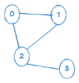
Q Knowledge Graph (QKG) can rank nodes, reshape graphs into perspectives, and grow neighborhoods around seed entities on graphs with billions of nodes and edges. QKG can manage this at scale because it treats the knowledge graph as sparse matrices, rather than as objects and pointers. Underneath the friendly Python API, this architectural choice turns large-scale graph analytics into linear algebra in a format that computers can store compactly, optimize aggressively, and execute at scale. You don't need to be an expert in sparse matrices to use QKG. However, understanding makes use of sparse matrices explains why QKG scales so well, and why it's built differently from a traditional graph database. It will also help you use QKG effectively and make the most out of it. The problem: Graphs don't scale neatly What is a graph? You could picture it as a big bag of node objects, each holding a list of pointers to its neighbors. This works for a few thousand nodes, but it falls apart at real world scale. A network resolved from customer data, corporate registries and transaction records can easily reach hundreds of millions - even billions - of nodes. Holding that many objects in memory on one machine can be inefficient, and "walking the graph" by chasing pointers becomes painfully slow when each step is a random jump around memory. Handling big graphs means storing them in a form a computer can process efficiently and at scale. Using linear algebra, it is possible to represent graphs in a matrix form. For example, take a small graph with four nodes and the edges . Figure 1 - Example graph with edges (0,1),(0,2),(1,2),(2,3) The undirected graph with four nodes and edges shown in Fig. 1 can be represented by the following adjacency matrix. The adjacency matrix is a grid with one row and one column per node, where a 1 in row i, column j means "there's an edge from i to j". This fully represents the graph structure, i.e. nodes and edges - no information is lost. And once a graph is a matrix, the whole toolbox of linear algebra opens up. Multiplying this matrix by a vector, for instance, is the same as taking one step along every edge at once - a single, batch operation instead of millions of individual pointers. Many node and relationship types, many matrices Real knowledge graphs are heterogeneous - they might mix individual, business and account nodes, connected by different relationships like owner, director and transaction. QKG handles this by storing multiple matrices, each representing a specific relationship between two nodes, also known as triplet. A triplet is a typed, directed relationship written as (source type, relationship, target type): individual-owner-account and account-transaction-account are two different triplets, and each gets its own adjacency matrix. Why sparse is the whole trick A graph with a million nodes has a million-by-million adjacency matrix, which is a trillion cells in total. Storing a normal (dense, filled with 0s and 1s) matrix in memory is simply too expensive. In real networks, however, the absence of edges (the 0s in the adjacency matrix) outnumbers their presence (the 1s). Each person knows hundreds of others, not millions. In transaction networks, each account is likely to transact with a small number of counterparties, rather than most accounts worldwide. The number of actual edges is tiny compared to the number of possible ones. In other words, the adjacency matrix is sparse - the majority of its entries are zero. A sparse matrix exploits this feature by storing only the non-zero entries - the connections that actually exist - and simply assuming everything else is zero. For a realistic graph that's a reduction of several orders of magnitude: from a trillion cells down to the relationships that are actually in your data. The same trick that shrinks the memory also speeds up the maths, because operations only touch the entries that are actually there. For example, if we consider the star shaped graph below, its adjacency matrix 𝐷, stored in a dense format, would be filled mostly with 0s. This representation needs 11 x 11 cells stored, hence 121 entries, mostly filled with 0s. As you can see, the storage cost is quadratic with the number of nodes of the graph. In a sparse matrix format, for example CSR (Compressed Sparse Row), we would store instead 3 arrays: 𝑆 = [1, 1, 1, 1, 1, 1, 1, 1, 1, 1, 1, 1, 1, 1, 1, 1, 1, 1, 1, 1] 𝐼 = [1, 2, 3, 4, 5, 6, 7, 8, 9, 10, 0, 0, 0, 0, 0, 0, 0, 0, 0, 0] 𝑅 = [0, 10, 11, 12, 13, 14, 15, 16, 17, 18, 19, 20] 𝑆 represents the non-zero values of the matrix (20 ones); I represents the column indices where these values are stored; 𝑅 represents the row pointers: for each row, it indicates where that row's values begin in the S and I arrays. The entries of row i occupy positions R[i] up to (but not including) R[i+1], so the number of non-zero values in row i is R[i+1] - R[i]. Its length is n + 1 (one entry per row plus a final entry equal to the total number of non-zeros, 20 here). For example, row 0 spans R[0]=0 to R[1]=10, so its non-zeros are the first 10 entries of S/I (columns 1 to 10); row 1 spans R[1]=10 to R[2]=11, a single entry at column 0. The storage cost using the sparse format is (2 x nnz + n + 1), where nnz is the number of non-zero values and n is the number of nodes in the graph. Compared to the quadratic cost of the dense format, the sparse format is linear in the number of nodes and non-zero values. In the example above, we only needed to store 52 values instead of 121, but this difference will be more extreme as the graph size increases. Similarly, and symmetrically to the CSR format, there is the CSC (Compressed Sparse Column) format, which stores the matrix by columns instead of rows. It also holds 3 arrays: S holds the non-zero values, read column by column; I now holds the row indices of those values (rather than the column indices); The pointer array R marks where each column begins in S and I. CSC is efficient for column-based operations, just as CSR is efficient for row-based ones. QKG handles these formats automatically, hence you don’t have to specify anything. This is the engine behind Q Knowledge Graph. Representing graphs as sparse matrices is what lets QKG hold enormous networks and run real algorithms over them efficiently, instead of storing graph objects with pointers that would result in out of memory errors. Algorithms become arithmetic Once your graph is a set of sparse matrices, many classic graph algorithms turn into short sequences of matrix operations. Perspectives - Using linear algebra, for example, it’s possible to reshape the graph by collapsing a multi-hop path into a single derived relationship. Chaining individual → owner → account → transaction → account → owner → individual into a direct individual-transaction-individual edge is a sequence of matrix multiplications (one per hop), with the results aggregated together. This lets the same underlying data foundation be reshaped for different business challenges, from large-scale analytics to graph machine learning, without ever duplicating the data. This process is detailed in the following Quantexa patent: Method and System for Generating at Least One Perspective of Knowledge Graph (No. US US18781012), which describes a scalable way of resolving perspectives from even the largest datasets by using lazy evaluation to chain operations together efficiently. Other QKG algorithms rely on sparse matrices, for example: Neighborhood expansion - growing outward from a set of seed nodes – this is a matrix operation: by multiplying the seeds’ neighbours vector by the adjacency matrix it’s possible to get all nodes one hop away; doing it twice will yield the nodes two hops away (the neighbors’ neighbors), and so on. The path queries defined in EgoBuilder do exactly this. PageRank – one of the best known centrality algorithms, originally developed by Google's founders to rank web pages. It works by imagining a random walker hopping along edges, and asking where they spend most of their time. PageRank simply measures where this walker spends most of their time, and ranks the nodes accordingly. Behind the scenes, working this out comes down to repeatedly multiplying a matrix by a vector - and because our matrix is sparse, each of those steps is fast and cheap. In general with QKG, instead of writing bespoke traversal code for each algorithm, whenever possible, it’s faster and more efficient to express algorithms using matrix-vector operations. Making it fast: switching backends Expressing algorithms as linear algebra has one more advantage: you can swap in whatever engine computes that linear algebra fastest, without changing the algorithm. QKG uses a pluggable backend for its matrix operations: SciPy (the default) - a mature, reliable sparse-matrix library, perfect for development and mid-sized graphs. GraphBLAS - a specification and library purpose-built for expressing graph algorithms as sparse linear algebra, offering serious acceleration on larger graphs. Summary To put all this together: A graph is an adjacency matrix, and a heterogeneous graph is a set of them, one per relationship type. Real networks are sparse, so storing only the edges that exist cuts memory by orders of magnitude. Algorithms like PageRank, neighborhood expansion and Perspective generation become sequences of sparse matrix operations. Those operations can run on an optimised backend, and distribute over Spark, so the same code scales from a laptop to a cluster. QKG's sparse-matrix architecture is designed for real-world data at enormous scales. This design is what lets the same graph logic run on a laptop or across a cluster, doing network operations at a scale that would overwhelm a traditional in-memory graph. If you'd like to see these ideas in action rather than in theory, head back to Creating and exploring a Q Knowledge Graph to run PageRank and generate Perspectives on a graph of your own.61Views0likes0CommentsDo Cycles Hide Risk? A Legal Hierarchy and Japan’s Keiretsu Networks Story
At Quantexa, we help organizations make more informed decisions and run analytical solutions at scale. And since any analysis is only as good as the data behind it, it all starts with a single, trusted view of your data, delivered through out-of-the-box Entity Resolution. We bring together fragmented information from multiple sources to reveal the relationships that matter. In this blog post, we explore shareholder weighted links to trace ownership stakes across corporate registry data, who owns whom, and ultimately, who controls a company. Quantexa Legal Hierarchy Legal Hierarchy was developed to answer that question, transforming disconnected corporate records into structured ownership networks that can be explored, analyzed, and understood. LH docs Ownership isn't a straight line. Company A may own Company B, which in turn owns part of Company C, creating relationships that are easy to understand in isolation but difficult to follow across an entire jurisdiction. Scale that to millions of entities and ownership links, and even seemingly simple questions become challenging: Who ultimately controls this company? Which organizations belong to the same corporate group? Are there hidden connections between two unrelated entities? Are there unusual ownership structures that could be risky? Legal Hierarchy helps answer these questions. Through LH, users can navigate ownership structures, identify controlling entities, trace relationships across multiple levels, and uncover patterns that would be difficult to spot from individual company records alone. But why does this matter? For the organizations we work with, banks, insurers, regulators, and government agencies, understanding who owns and controls a company sits behind some of their most important decisions. On the risk side, it helps them know who they are really dealing with. Before lending money, onboarding a client, or approving a payment, they need the full picture: who ultimately owns the company, which group it belongs to, and whether that group is exposed to sanctions, fraud, or financial crime. A company can look perfectly safe on its own and turn out to be risky once you see the entities standing behind it. Legal hierarchies also help measure exposure: a bank might lend to twenty companies that all belong to the same group, which is a much bigger bet than twenty separate ones. On the opportunity side, the same view pays off. Knowing a client's full corporate group helps an organization understand the whole relationship, spot new business, and serve customers as one connected group instead of a pile of disconnected accounts. Running Legal Hierarchy across a jurisdiction often begins with data that appears perfectly valid on the surface. However, once ownership relationships are connected and visualized as a network, unexpected patterns can emerge. What seemed like a straightforward corporate structure can reveal relationships that are difficult to explain, unusual ownership arrangements, or configurations that warrant further investigation. Figure 1: Japan and several well-known tax havens show the same pattern: normal direct ownership, but a sharp rise in indirect owners and cycles This is exactly the case. All the countries looked exactly like what we expected: small, tidy ownership trees, barely any cycles. About one direct owner, one indirect owner, and well under one entity per hierarchy caught in a loop. However it’s difficult to not look at Japan. The direct owners were normal, about the same as the rest of the countries. But look one step further, and it all explodes: nearly ten indirect owners per company instead of one, and around nine entities per hierarchy caught in an ownership loop. A jump that big isn't noise or a broken pipeline, it's telling us something real about the way Japanese companies own each other. So we went looking for why, and the same answer kept coming back: keiretsu networks. Keiretsu Networks A keiretsu network is a system of independent Japanese companies that work closely together and own small shares in each other to support mutual business success. They grew after World War II to help rebuild the economy and protect member firms from outside market shocks and hostile takeovers. This is the evolution of the zaibatsu networks that used to be the single-family holding companies, during the Cold War, these firms were reorganised using cross-shareholding and main banks instead of family control, giving rise to the current keiretsu networks. We have different types of keiretsu: Horizontal groups: Link companies across many different industries like finance, trading, and manufacturing, usually centered around a major bank (e.g., Mitsubishi). Vertical groups: Connect a major manufacturer down to its specific supply chain, parts makers, and local distributors (e.g., Toyota) Do the Keiretsu networks hide risk? Can we then confirm whether Keiretsu networks hide risk or not? For example, Toyota is one of the most famous companies in the world and one of the largest Keiretsu groups in Japan. If we do some expansions at the Quantexa UI, we got: Figure 2: Toyota entity-to-entity network with multiple ownership cycles, a textbook keiretsu where the shareholding arrows loop back to where they started. Looking at its ownership network, would you be able to identify any risk? Probably not. At first glance, it looks like a dense collection of companies and relationships. This is where Legal Hierarchy helps. By building the parent hierarchy, the underlying ownership structure becomes much clearer, making the close and interconnected relationships easier to spot. ed by ownership. The highlighted path shows the Denso cycle. Toyota looks like a textbook case of the "weird behavior" we found in Japan. Toyota owns Denso and Toyota Industries, and both of them own a small part of Toyota back. That is a cycle: A owns B, and B owns A, the kind of loop that makes a hierarchy look suspicious So, is it risky? Not really. This is just how a vertical keiretsu works. Toyota keeps long-term relationships with its key suppliers, and these small cross-shareholdings exist to protect those relationships, not to hide who is in control. But now picture the same shape in a very different setting. Imagine a handful of companies registered in places known for secrecy, with no real employees and no real business, that own each other in a loop: A owns B, B owns C, and C owns back into A. On paper, no single person owns enough of anything to look like the one in control, and that is the whole point. The loop isn't there to hold a supply chain together, it's there to break the trail, so nobody can easily work out who really owns or benefits from the money moving through it. That kind of circular structure is a classic red flag for hiding the real owner behind a company, whether to launder money, move funds past sanctions, or disguise who is actually in charge. The shape on the graph is almost identical to Toyota's. The difference is everything around it. Toyota's cycle is made of real, well-known companies with decades of business between them, and the cross-shareholdings are small and out in the open. The suspicious version is built from empty shells in opaque jurisdictions, designed precisely so the ownership can't be followed. And this is the tricky part: the same pattern can mean two very different things. It can be a deliberate attempt to hide who is in control, like the shell-company loops above, or a perfectly legitimate structure, like the one that holds Toyota's group together. The shape alone can't tell you which. There is also a third case, and it is the most subtle one. Sometimes the structure is legitimate, but the culture around it still lets things go wrong. Toshiba is a good example. Between 2008 and 2014, Toshiba overstated its profits by around ¥151.8 billion, in one of the biggest accounting scandals in Japanese history. It wasn't a single trick but a mix of accounting tricks across different business units, booking profits too early, pushing losses into later years, and recording revenue before the work was really done. https://www.nippon.com/en/in-depth/a04802/ ) The fraud only came out in 2015, after a whistleblower reported it to Japan's financial regulator, and it ended with the CEO and eight senior executives resigning. However, the keiretsu structure didn't cause the Toshiba fraud, and it wasn't how the numbers were hidden, but the culture around it, where big shareholders rarely challenge management, is part of why it went on for years before anyone stopped it That's where Legal Hierarchy fits. LH is very good at one thing: showing these structures at scale, so nothing stays hidden inside millions of records. It shows you the cycles, the unusual owners, the hierarchies that don't look normal. What it can't do is decide, by itself, whether a structure is risky. That still needs a person, an expert who knows the jurisdiction, the industry, and, in this case, the story behind the keiretsu.41Views4likes0Comments
Wealth Management Lead Identification
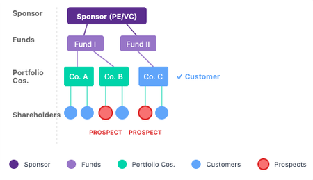
Wealth Management Lead Identification: Using Graph Data Science to Find High-Value Prospects How Quantexa graph analytics uncovers hidden opportunities in Private Equity ecosystems All names, companies, and figures in this article are synthetic data generated for illustration purposes. Any resemblance to real individuals or organizations is coincidental. The Problem: Valuable Prospects Hidden in Complex Ownership Structures Wealth managers know that relationships win business. The most valuable prospects often sit inside sponsor ecosystems - Private Equity firms, Venture Capital, and similar investment networks. These individuals have substantial wealth tied to portfolio companies but finding them and reaching them through warm introductions is extraordinarily difficult. Why? Because ownership structures are deeply complex. Consider a typical scenario: A Private Equity firm owns a fund, which owns another fund, which in turn owns a portfolio company. This chain can go five, six, or more layers deep. Within these structures, high-net-worth individuals hold indirect ownership stakes that translate to significant wealth - but are nearly impossible to trace manually. Several challenges make this difficult: Sponsor ecosystems are large, complex, and computationally expensive to map out Connecting internal and external data for both people and businesses is difficult Ownership chains run deep - calculating indirect ownership requires sophisticated algorithms Scaling analytics to prioritize focus and automatically identify the highest-value opportunities is hard Manually tracing these connections is slow, inefficient, and often misses the most valuable indirect relationships entirely. The Solution: A Three-Step Graph Data Science Approach Our approach follows three key steps, building on Entity Resolution as the data foundation: Knowledge Graph Construction - Structure unified data into a Quantexa Knowledge Graph Hierarchy Algorithm - Calculate true ownership stakes across all layers Lead Scoring - Prioritize prospects using graph-derived metrics Step 1: Building the Knowledge Graph After Quantexa Entity Resolution creates a unified view of the different entities in the data, like people and businesses, we structure this data into a Knowledge Graph. The Knowledge Graph maps out relationships across the entire dataset – in our case businesses and individuals and how they connect. Think of it as taking all the fragmented data about companies, funds, and people, and turning it into a single, connected picture. Every shareholder relationship, every board seat, every subsidiary - all visible in one place. A visualization of theKnowledge Graphcreated from corporate registry and customer data Businesses, individuals, places, events and how they connect — across the entire dataset Ownership Ontology: Simplifying for Scale To make the solution scalable and target it to our problem, we use Knowledge Graph Ontologies/Perspectives to collapse shareholder and subsidiary relationships into a single "ownership" edge. This simplification: Reduces computational complexity Allows downstream analytics to focus on what matters - the ownership chain Eliminates the need to traverse every relationship type in the full graph The result is a complete map of who owns what across the entire ecosystem. Step 2: The Hierarchy Algorithm - Uncovering Hidden Ownership Here's where it gets interesting. Looking at the data, we see direct shareholder information i.e. Sarah Mitchell shows up as a 8% shareholder in a company called Quantum Shield. But Quantum Shield sits inside a Private Equity ecosystem - owned by funds, which are owned by other funds, which trace back to a major sponsor. When we follow the ownership chain all the way through, Sarah's 8% stake connects her to hundreds of millions in value across the portfolio. The Hierarchy Algorithm propagates ownership through every layer, answering: "Who really owns what, when you follow the money all the way through?" Suddenly, hidden relationships surface: Someone with "just 8%" of one company has indirect exposure worth hundreds of millions A prospect buried four layers deep is connected to companies you already serve Warm referral paths appear that were invisible before Step 3: Lead Scoring - Prioritizing with Graph Metrics Now that we understand the full ownership picture, we can identify and prioritize potential leads using three graph data-driven scoring models: Estimated Net Worth Formula: Σ (Ownership % × Company Valuation) Using the indirect ownership percentages calculated by the hierarchy algorithm, combined with company valuations, we estimate each individual's net worth derived from their portfolio holdings. Example: 16% indirect ownership × $3,500M company valuation = $560M estimated net worth This provides a baseline understanding of potential wealth. Relationship Strength This score measures a prospect's connections to existing customers, considering: Number of shared connections Roles (e.g., co-directors, board members) Recency of relationships A high relationship strength score means stronger referral paths and higher likelihood of conversion. Prospects connected to multiple existing customers through meaningful business relationships are more likely to respond to warm introductions. Network Influence This centrality metric measures how connected an individual is across the entire Knowledge Graph - not just within one sponsor ecosystem. Highly influential individuals: Sit at network hubs connecting multiple businesses Have higher lifetime value Offer greater future referral potential The Results: Actionable, Prioritized Leads Below is a snapshot of the top results - for each lead, we provide: Estimated net worth derived from indirect ownership calculations Network influence score based on graph centrality Relationship strength to existing customers The exact referral path - which existing customers can provide warm introductions Prospect Portfolio Company Sponsor Est. Net Worth ($B) Network Influence Relationship Strength Referral Path SARAH MITCHELL Quantum Shield Pinnacle Horizon Ventures LLC 0.34 0.20 0.24 Pinnacle → Quantum Shield → JOHN FITZGERALD CONNOR OBRIEN Quantum Shield Pinnacle Horizon Ventures LLC 0.23 0.16 0.16 Pinnacle → Quantum Shield → JOHN FITZGERALD ETHAN HARRIS DataFlow Systems Suncrest Solar Projects Ltd 0.08 0.05 0.01 Suncrest → DataFlow → MICHAEL BROWN, EMMA DAVIS OLIVIA MARTINEZ EduTech Platforms Suncrest Solar Projects Ltd 0.08 0.02 0.01 Suncrest → EduTech Platforms For our top prospect, Sarah Mitchell, we not only see her high net worth score but also the exact referral path: an existing customer, John Fitzgerald, along with the portfolio company where they're connected (Quantum Shield). This gives the relationship manager everything needed to make an informed, warm approach. Visualizing the Ownership Flow The hierarchy graph visualization shows the complete ownership chain from sponsor to portfolio company to prospect: This produces a visual hierarchy showing: Pinnacle Horizon Ventures LLC (Sponsor) at the top Fund structures (Pinnacle Climate & Renewal Fund, Pinnacle Digital Frontier Fund) Portfolio companies (Quantum Shield, Synapse AI, Circulus Materials, etc.) Individual shareholders with their ownership percentages Existing customers highlighted for referral identification Technical Stack Quantexa Knowledge Graph (QKG) - Graph construction and ontology management Legal Hierarchy Algorithm - Indirect ownership propagation PySpark - Distributed processing for scale Graph Centrality Algorithms - Network influence scoring This approach demonstrates how graph data science transforms complex relational data into actionable business intelligence. By combining Knowledge Graphs, hierarchy algorithm, and graph-based scoring, wealth managers can identify high-value prospects they would otherwise never find - and reach them through warm, trusted relationships.78Views0likes0Comments